Irrotational and rotational Flows
NARRATIVE -
CONNECTION TO THE TEXT
Chapter 1, Sec.1.3 Rectangular system of coordinates, the Curl operator of
Eqn. 1.12 acts on the velocity field to produce a new vector field called the
fluid vorticity ω. Vorticity has the magnitude of twice the local fluid
rotation rate and its direction aligned with the local axis of rotation. For
flow in the x-y plane.
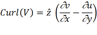
It is straightforward to see that Curl(V) involves rotation by
investigating the case of steady uniform fluid rotation in the x-y
plane, as shown in Fig. 1.1 (left panel). Take the center of rotation to be at
the origin and the initial position of a fluid particle to be at x = R, y =
0. The trajectory of the particle is then x = R cos(ωrott)
and y = R sin(ωrott), where ωrot
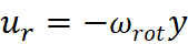
is the angular velocity (rotation rate) in radians per second. In this case u
= dx/dt = −ωroty and v = dy/dt = ωrotx.
Taking the curl of this velocity field gives 2ωrot for
all x and y, or twice the fluid rotation rate. In the general
case, there can be local patches of rotation embedded in an otherwise
irrotational flow.
Another way of understanding this example of uniform rotation is through Stokes
Theorem, which relates the line integral of a vector function F along a
closed loop (in this example a circular loop) to the total Curl(F),
enclosed within the loop (see image below)
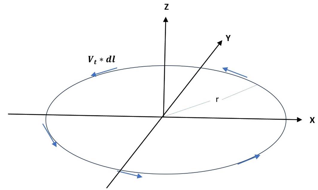
The line integral of the tangential velocity Vt along the
full loop is 2πrVt and the enclosed Curl(V), or ω, is πr2ω, Solving this
gives Vt=1/2rω, or Vx = -1/2rωsin(ωrot t), Vy
= 1/2rωcos(ωrott)
The cross-product term in Eq. (1.12) is therefore closely related to the
transport of vorticity. There can be surprises however: the flow field in Fig.
1.1 (right panel), defined as u=α x, v=−α y, w = 0,
would appear to possess vorticity but is actually irrotational since Curl(V)
= 0 everywhere. When fluid motion is irrotational, Eq. (1.12) simplifies to
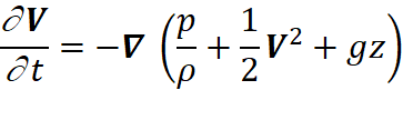
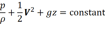
In this case, the nonlinear
term is interpreted as a change in kinetic energy with position, see Kundu and
Cohen (1990). Note that in the steadystate case where ∂V/∂t = 0, above
Eq. reduces to the Bernoulli equation
Model Description
·
The
animation or movie below depicts the transition from irrotational (left panel)
to rotational flow (right panel) motion of a fluid. A smooth ramp function
(sigmoid-like transition from 0 to 1) makes the transition of the fluid states.
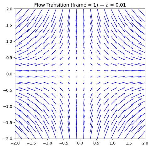
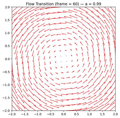
Figure-movie 1.1 -Left panel: uniform irrotational.
Right panel: rotational flow
<Click HERE
to WATCH Irotational to rotational transisition_1.mp4>
Model summary
Transitioning Flow:
Irrotational → Rotational. Figure-movie 1.2 sigmoid transition function
(ramp) for the transition parameter (a) see ramp function in python program
(rotational.py). u and v are x-direction and y-direction
horizontal velocity field.
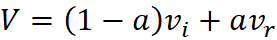
The Velocity field
functions for the irrotational field is defined as
Where x and y
represent the x-coordinate and y-coordinate respectively.
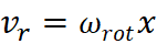
On the other hand,
the velocity field function for the rotational field is defined as
The transition
between irrotational to rotational flow is achieved by using a smooth ramp
function (sigmoid-like transition from 0 to 1) thus

Where f is the
movie frame count and f_max is maximum frame count (60), see
Figure-movie 1.2
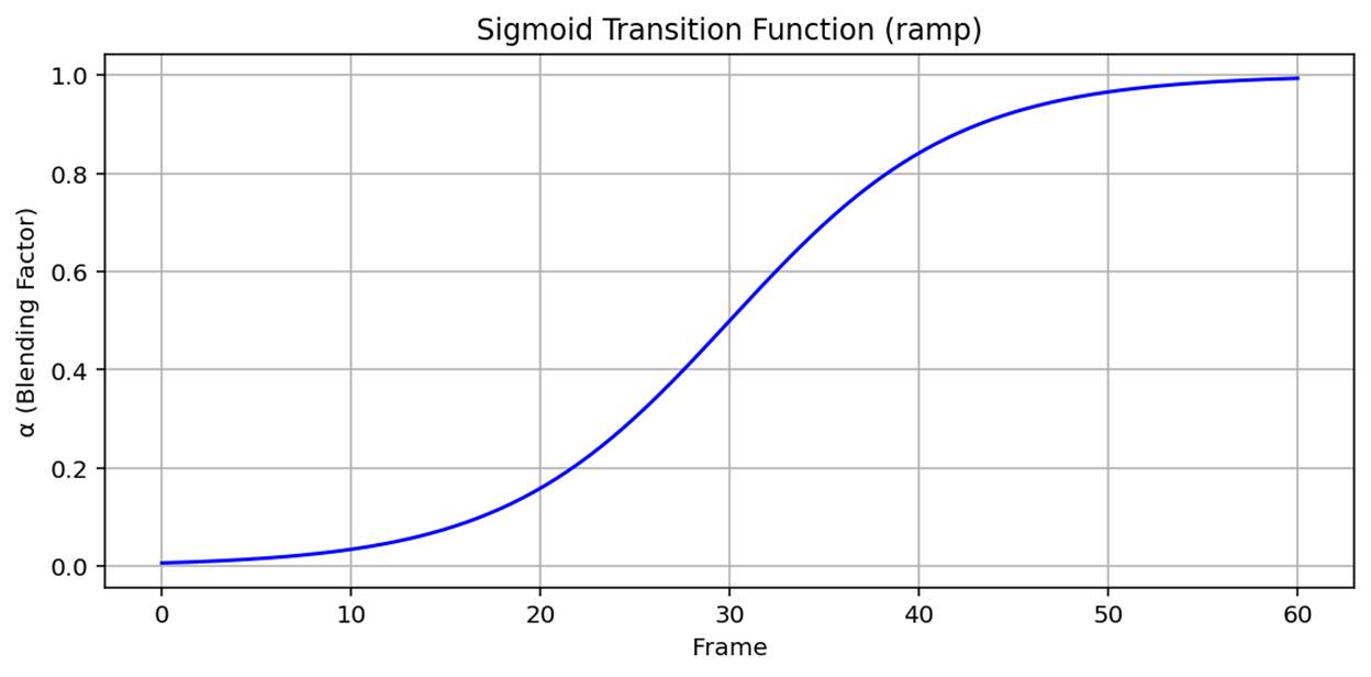
Figure-movie 1.2 <96> Transition ramp from irrotational
to rotational
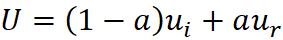
The
transitional velocity from irrotational to rotational in the movie is then
calculated as:
Chapter 2
LARGE AMPLITUDE OSCILLATIONS IN A PARABOLIC TROUGH
NARRATIVE -
CONNECTION TO THE TEXT
Chapter 2, Sec.13.2
describes oscillatory fluid motion within a parabolic cross section trough.
There are several analytical solutions to the depth averaged equations of
motion and continuity under these conditions. This offers a useful comparison
with NLSW model results. Various runup / rundown algorithms and sea level
reconstructions can be tested under large amplitude wave conditions. Two full
cycles of the two lowest modes oscillation are animated here – accompanied with
an assessment of model errors accumulated over a span of 5 cycles
Model Description
·
The
animations below depict motion of the two lowest “slosh” modes. Dimensions of
the trough are as described by Eqn. (2.123) in the text and shown in Figure-movie
2.1.
·
A
1-D, non-linear shallow water wave model is used to solve numerically for u
(x, t) and ζ(x,t). To be consistent with the analytic results
however, bottom friction is dropped.
·
Spatial
step size ∆x is 100 m, time step is .005 s.
·
Position
along the x axis is denoted by x = ∆x * i where i = 1, 2, 3,
4, …….., 1601
·
Animation
frames were generated at 25 s intervals to depict two full periods of
oscillation (t = 1998 s for the lowest mode, and ~1152 s for the next higher
mode)
·
The
initial conditions for the two animations are:
o Mode 1: U(x, 0) =
0, ζ(x, 0) = .01*x
o Mode 2: ζ(x, 0) = 0,
U(x, 0) = 6.34×10⁻⁴s-1*x,
·
Equations
of motion and continuity are modeled with Eqns. (2.121) and (2.122)
respectively as displayed in the text. Flux formulations for sea level updates
(Eqn. 2.102) are used to insure conservation of mass.
·
The
runup algorithm is shown in Fig. 2.32 of the text and the rundown algorithm is
shown in the Fortran code “snippet” preceding the figure
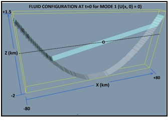
Figure-movie 2.1 - model domain with mode 1 initial
conditions
<Click HERE to WATCH Thacker_1.mp4>
<Click HERE to WATCH Thacker_2.mp4>
Model summary
Sea level dynamics
and oscillation periods for both modes track closely with analytic expectations
(Figure-movie 2.2 below). The period of oscillation for mode 1 is 1998 s and
is identical to numerical results even after 5 cycles of motion. The maximum
modeled sea level slope drops by .06 % during this same time. This is expected
as the numerical system slowly “runs down”.
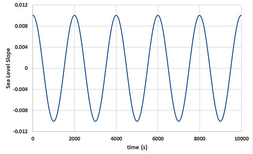
Figure-movie 2.2 - sea level slope - Mode 1
Accumulated errors in the mode 2 model for system energy and
mass are plotted below in Figure-movie 2.3
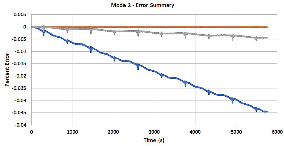
Figure-movie 2.3 Red curve: mass error, blue curve: total system energy
error using piecewise constant sea level reconstruction, gray: total system
energy with piecewise linear sea level reconstruction
Mass
is conserved throughout the 5 cycles of oscillation. Energy (kinetic +
potential) is slowly lost however. The error spikes occur at moments of
maximum runup and minimum rundown.
Dam-Break Problem
NARRATIVE -
CONNECTION TO THE TEXT
The dam-break problem is one
of the oldest hydraulic problem whose solution derived by the method of
characteristics is given below in the left panel. The dam breaks
instantaneously at t=0 and generates two waves: a negative wave propagating
into the fluid and a positive wave propagating over the dry bed. The wave front
of the non-viscous fluid propagates over the dry-bed with speed  which is two times
greater than the wave front speed moving in the negative direction. At the dam
site, the water depth drops instantaneously to a constant value of
which is two times
greater than the wave front speed moving in the negative direction. At the dam
site, the water depth drops instantaneously to a constant value of  where
where  is the initial depth,
(Figure-movie 2.4 left panel).
is the initial depth,
(Figure-movie 2.4 left panel).
In the right panel the
analytical solutions (continuous lines) and numerical solution have been
compared. Although results are quite good, a magnified picture of the free wave
profile shows that the numerical solution profiles lag slightly behind the analytical
profile. The computations presented in the right panel are elucidated in Chapter
2. They are based on the finite-difference approach and a special algorithm for
the runup.
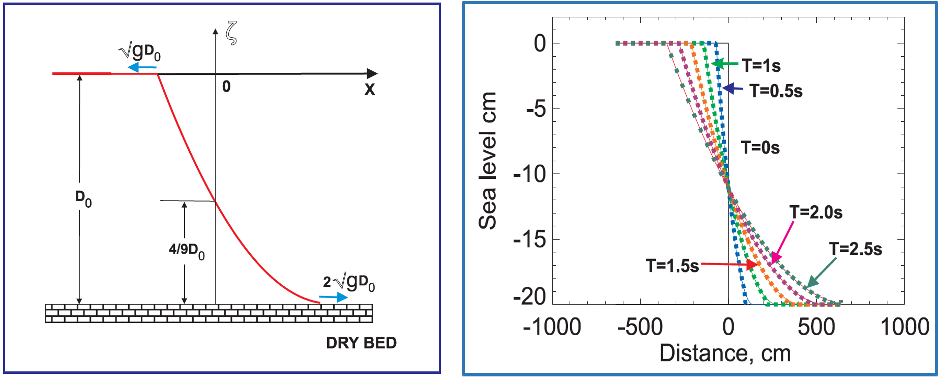
Figure-movie 2.4 – Dam break problem:
left panel analytical solution, right panel numerical solution.
Below we present two movies
which results from the dam-breaking solution by the FNS-VOF Model, which is
Full Navier-Stokes equation aided by the Volume of Fluid method. (See Chapter
6, Sec. 6.2.3). This method solves for two-dimensional fluid flow with tracking
of the free surface. The free surface of the fluid is described by the discrete
VOF function; this approach was conceived way back by Nichols and Hirt (1975).
Model Description
·
The
animations below describe the dam break problem using NVS-VOF model and
compares its solution with analytical (Figure-movie 2.5) and lab experiment
(Figure-movie 2.6)
·
The
NVS-VOF 2-D model solves vertical and horizontal motion. Velocities u, w
are solved by the two step methods for the solution of the pressure field. The
free surface is determined based on the VOF function which is defined by the
fraction of fluid in the computational cells.
·
Spatial
step along the horizonal and vertical is 0.0025 m and time step is 2.0e-4 s.
·
Density
is 1000 kg/m3 and the dam height is ho= 2.0m, for Figure-movie
2.5 and ho= 0.2m, for Figure-movie 2.6. The motion of the gate in
the Figure-movie 2.5 is instantaneous and in the NVS-VOF vs lab experiment is
given by z(t)=23.6t2+0.134t where t is time in s.
·
The
initial conditions for the dam break problem are:
o Figure-movie 2.5, u(x, y) = 0, w(x,
y)
= 0 and ho(-10 <x<0m) = 2.0m
o Figure-movie 2.6, u(x, y) = 0, w(x,
y) = 0 and ho(-7.5<x<0m) = 0.2m
·
Equations
of continuity and motion are modeled with Eqns. (6.10 ) and (6.11) respectively.
The free surface of the dam break fluid is modeled by the discrete VOF scheme,
Eqn (6.16) and the  function.
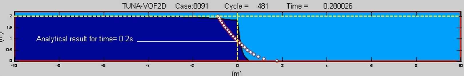
Figure-movie 2.5 NVS-VOF numerical solution versus
analytical solution.
Click HERE to
WATCH case_0091.mP4
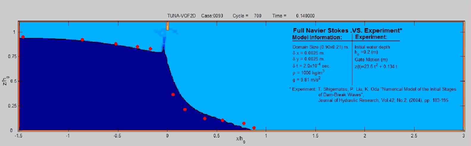
Figure-movie 2.6 NVS-VOF numerical solution versus lab
experiment, Shigematsu et.al., 2004.
<Click HERE to WATCH case_0093.mp4>
Model summary
From above
experiments it is evident that initial phase expressed by the analytical
solution is not well reproduced (which is expected), however as time progresses,
better agreement is observed. It is also noticed that in the lab experiment the
effect of the gate motion plays an important role at the initial phase and model
result gets better agreement as time advances. The speed of removing the gate
may also play an important role.
Reverse FAULT SOURCE AND INITIAL COASTAL RECESSION Vs
INUNDATION
NARRATIVE -
CONNECTION TO THE TEXT
For the Indian Ocean
tsunami, first wave arrivals at coastal points east of the source tended to be
troughs, while those to the west were crests. The ocean bottom deformations
used as sources for both the IOT and the KIT show a similar pattern of uplift
and down drop (Figure 3.9 from textbook for the IOT source deformation
contours). Representing the initial wave as a “copy” of the bottom deformation
as indicated in Figure-movie 3.1, and then expressing this as a sum of right
and left traveling wave as in Chapter 2, Eqn. (2.7) offers an explanation of
the signs of these first wave motions at coastal points.
Model Description
·
The
animation depicts the effect of a simplified “dipolar” earthquake source which
includes both down drop and uplift within the fault zone. This is commonly seen
with reverse or thrust fault mechanisms as tsunami sources. The resulting wave
dynamics show how coastal points at opposite sides of a fault can record
opposite senses of “first wave motion”.
·
This
is a 1D, transient shallow water wave model u (x, t) and ζ(x, t)
– with no non-linear terms. Depth is uniform at 1000 m.
·
Spatial
step size ∆x is 1 km, time step is 1 s.
·
The
position along the x axis is denoted by x = ∆x * i where i =
1, 2, 3, 4, …….., 1000
·
The
earthquake source is confined to 400km < x <600km, with uplift rise time
(t_max) of 10 s, width (l) = 200 km (centered at xo = 500 km), and maximum
uplift (ho) of 2 m. The
source is modeled as  for 0 < t < t_max.
·
180
animation frames were generated at 25 s intervals - giving 1.25 hours of wave
evolution. The animation rate is slowed by 25X during uplift (0 < t <
t_max) so the viewer can visualize the otherwise near-instantaneous source in
action.
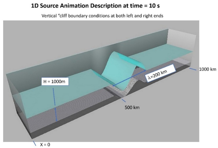
Figure-movie 3.1 1D source animation with left and
right traveling waves.
<Click HERE to watch movie (ReverseFaultSource.mp4)>
Model summary
Sea level at three
times (Figure-movie 3.2): blue at t_max (10s), red at 2500s, and grey at 4800s. Note the opposite
polarities of the wave arrivals at x = 0, and 1000 km at t=4800s. The lack of
spread or drop in amplitude of the initial sea-level deformation (blue curve)
shows that the uplift can be treated in this case as nearly instantaneous.
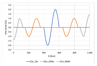
Figure-movie 3.2 1D source snapshots of wave
approaching left and right coasts. Blue, initial wave; red, open ocean and
gray, wave arriving coasts.
St. Augustine Volcano SOURCE, Generation and Maximum wave
amplitude in Cook inleT
NARRATIVE -
CONNECTION TO THE TEXT
The simulation of tsunami caused by landslide, presented in
Chapter 3.14, is further explained by considering the eruption of the Mount St.
Augustine volcano in 1883. During the eruption, a portion of the volcano
collapsed into the shallow water of Cook Inlet (Kienle et al., 1987).
Model Description
A numerical model was used to calculate the tsunami
generated by the debris flow from the volcano's collapse. The source of debris
is located on the volcano's eastern side, and Figure-Movie 3.3 provides the
basic parameters of the slide.
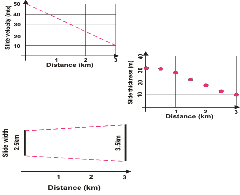
Figure-movie 3.3. Slide velocity, thickness and width
as a function of the distance for the eastern St. Augustine slide.
The distance of 3km in this figure describes the travel
distance of the slide from the time it entered Cook Inlet water. Along this
distance, the travel velocity of the slide diminished from 50 m/s to 10m/s, its
thickness along the center of the slide also diminished from 30m to 10m, while
the slide width increased approximately from 2.5km to 3.5km. This debris flow
was simulated as a progressive flow of the bottom uplift, which imparted motion
to the water column.
The tsunami's generation and propagation are calculated
using a set of equations of motion and continuity for the long wave equations.
The numerical form of these equations and appropriate boundary conditions for
the land/water and water/water boundaries are given in Chapter 4. The
finite-difference equations are solved in the spherical system of coordinates
with the grid spacing of 1 minute along the E-W direction and 0.5 minutes
along the N-S direction. The Cook Inlet domain depicted in Figure-movie 3.4 spans
from 58 50'N to 61 50'N and from 154 18'W to 148 18'W.
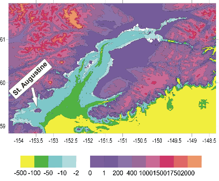
Figure-movie 3.4. Bathymetry (negative) and relief
(positive) of the Cook Inlet domain used in
numerical computations. Numbers are in meters.
The first result of numerical computation given in Figure-movie
3.5 defines travel times to various locations. Tsunami travel time to Homer is
close to 75min, while travel time to Anchorage is around 4 hours.
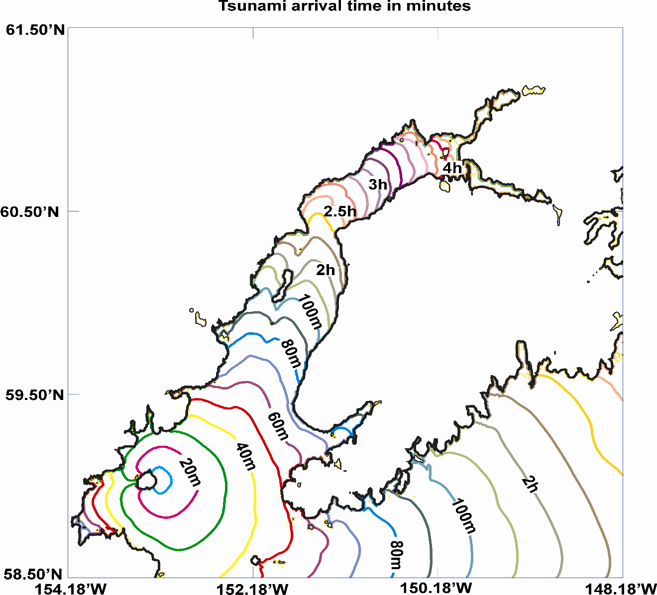
Figure-movie 3.5. Tsunami arrival time for the
eastern slide.
Figure-movie 3.6 describes the contours of the maximum
tsunami amplitude. This is the greatest wave height during the 5 hours of the
process. Usually, the maximum amplitude occurs at the different grid points at
different times. The spatial distribution of the maximum amplitude defines the
directional properties of the tsunami source; therefore, the maximum in Figure 3.6
is directed eastward, away from St. Augustine. While propagating towards the
shorelines, the tsunami amplitude is amplified along the peninsulas and ridges.
Westward from St. Augustine in the shallow waters of Kamishak Bay, tsunami
amplitude is
dissipated through the bottom friction.
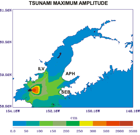
Figure-movie 3.6. Maximum tsunami amplitudes in
centimeters. Abbreviations: APH, Anchor Point –Homer; SEB Seldovia-English
Bay; ILV, Iliamna Volcano.
The strongest amplification occurred along the
Seldovia-English Bay shoreline, up to approximately 2.5m (Figure-movie 3.6).
Amplitudes of about 2m occur along Anchor Point -Homer (APH) shoreline and
along Iliamna Volcano (ILV) shoreline. This amplification is essential for the
coastal communities along the eastern shore of Lower Cook Inlet as the tsunami
travels to SEB in 50 min and to APH in about 75 min; therefore, warning time
for these communities is relatively short.
We have produced two movies to describe better the above
results. The movie titled Maximum amplitude (Figure-movie 3.7) checks the
amplitude in every grid point while the signal propagates from the source, and
only the maximum wave height is retained. The final distribution of the maximum
wave height is also plotted in Figure-movie 3.6.
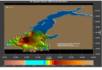
Figure-movie 3.7 Maximum wave amplitude recorded in
time due to the flank collapse of the St Augustine volcano.
<Click HERE to watch movie (Maximum_Amplitude.mp4)>
The propagation in time of the tsunami signal is given below
(Figure-movie3.8) in the movie titled amplitude in time. Out of this movie, the
tsunami arrival time is calculated and plotted in Figure-movie 3.5.
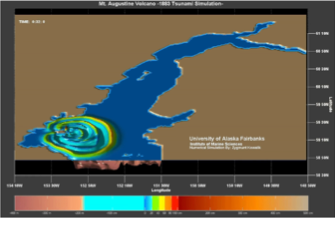
Figure-movie 3.8 Tsunami wave propagation in time due
to the volcano flank collapse of the St Augustine volcano
<Click HERE to watch movie (amplitude_in_time.mp4)>
Model summary
Numerical computation shows travel time and maximum
amplitude as important parameters for hazard mitigation in the coastal
communities. Computations delineate the important role of bathymetry in tsunami
coastal amplification where submerged peninsulas or ridges serve as tsunami
guides.
References:
Kienle, J., Z. Kowalik, and T. Murty. 1987. Tsunami
generated by eruption from Mt. St. Augustine volcano, Alaska. Science 236:1442-
GLobal Tsunami Propagation
NARRATIVE -
CONNECTION TO THE TEXT
Chapter 4 presents
numerical tools for the investigation of tsunami propagation in the World Ocean
based through modeling the Indian Ocean Tsunami (IOT) of December 2004, the
Kurile Island Tsunami (KIT) of November 2006 and the Japan Tsunami (JT) of
March 2011.
Model Description:
The global model for
the IOT, 2004 was formulated in spherical polar coordinates. Grid points were
assigned to the World Ocean from 80 south latitude to 69 north latitude with a
spatial resolution of one minute. This resulted in a massive 220 million grid
points. Using Whitmore’s source function that showed the sea floor’s tectonic
activity and the subsequent vertical displacement of water. Energy flux was
implemented to investigate energy transfer from the tsunami source across the
India Ocean to the Atlantic and Pacific Oceans. The sheer size of the
computational domain of the global model required a parallel code. The entire
domain was split along meridians into 40 subdomains and was run on a
supercomputer, Cray X1 (Artic Research Supercomputer Center, University of
Alaska, Fairbanks). The computational task took less than 10 hours on 60
multi-streaming processors, just under half the machine maximum capability.
The Kurile Island
Tsunami, 2006 model was also formulated with one minute grid spatial resolution
(7800x2640 grid points). The source function is given in Figure 4.22. The
tsunami spreads along the entire Ocean Pacific, but the main tsunami signal was
confined in the northern hemisphere. Several important bathymetric features
(Guyot inset), and scattering dynamics (energy flux) are
discussed further to understand the Kurile Tsunami transformation.
Model SUMMARY
Indian Ocean Tsunami, 2004
The movie below depicts
propagation of tsunami only in the Indian Ocean in December 2004 while looking
from above at the ocean surface. The source function, i.e. the bottom uplift
has been described in Chapter 3, Sec.4. The movie (Figure-movie
4.1) is strictly related to the Chapter 4, Sec.3. The movie
shows wave propagation in real time. Initial bottom uplift generates two
wave-systems, one traveling to the East into Indonesian Islands and the second
wave propagates to the West towards India and Maldives Island. The wave moving
to the India and Sri Lanka is strongly reflected from Sri Lanka sending tsunami
towards South-East. The reflected wave from the Bay of Bengal again is directed
towards south, thus this signal will combine with Sri Lanka signal and travel
along deep ocean ridges towards Antarctica. The wave front directed towards
Maldives Islands is transformed into three different signals: the reflected waves
which join signals from Sri Lanka and Bay of Bengal. The trapped signal which
stays around Islands and the passing signal which continues its travel towards
Arabian Peninsula, Africa and Atlantic Ocean. It is interesting to notice that
the wave front blocked by Maldives converges behind the Islands resulting in
the focusing tsunami energy by this long island chain (see wave front west of
the Maldives). One of this secondary energy beams directed towards the coast
of East Africa caused sea level rise to 3.3 meters. Both computations and
observations demonstrate a significant increase of the tsunami amplitude of
up to 1.5 m at the coast of Arabian Peninsula. The movie was produced at the
Arctic Research Supercomputer Center of University of Alaska, Fairbanks.
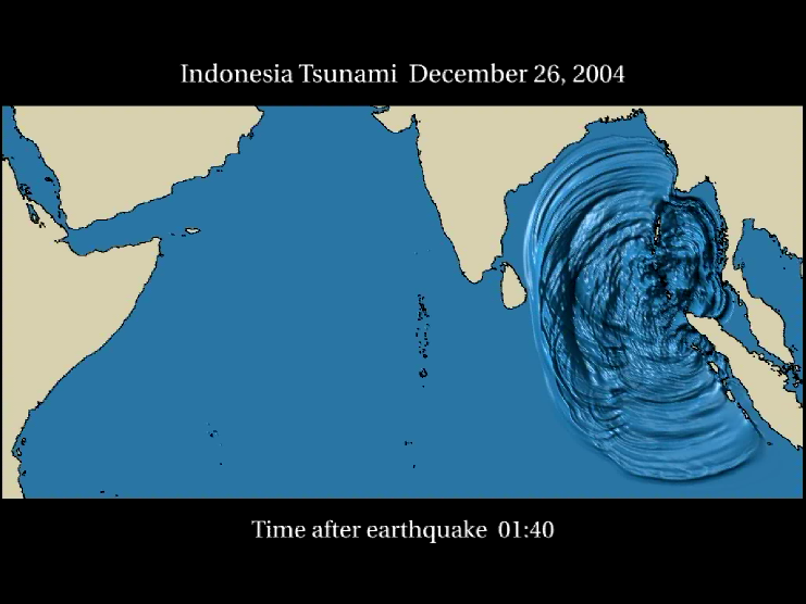
Figure-movie 4.1 Indonesia tsunami Dec. 26. 2004 Indian
Ocean Tsunami animation.
<Click HERE to watch movie (top_2fps1.mp4)>
Global Indian Ocean Tsunami,
2004
The movie below
(Figure-movie 4.2), depicts the generation of the tsunami in the Indian Ocean
in December 2004 and subsequent tsunami propagation in the entire World Oceans.
The source function, i.e., the bottom uplift, has been described in Chapter 3, Sec.4.
The movie is strictly related to Chapter 4, Secs. 5 and 6, where the physics of
propagation is explained based on the calculated energy flux through cross-sections
between Africa and Antarctica and Australia and Antarctica. The movie shows
wave propagation in real-time. Initial bottom uplift generates a
two-wave-systems, one is traveling to the East into Indonesian Islands, the
second wave propagating to the west towards India, Maldives Islands, and the
Atlantic Ocean, and the south towards Antarctica and the South Pacific Ocean.
It is interesting to see that travel routes in the Global Ocean are not
uniquely defined; therefore (important for the tsunami warning), travel time is
also not uniquely defined. For example, the wave traveling to Alaska can arrive
via Indonesian Islands in the shortest time; fortunately, with low energy. The
second route leading via South Pacific (along ridges) will bring a tsunami a
few hours later but with a much stronger signal. Observing the wave pattern
between South America and Antarctica, one can see that the
above wave is influenced by the signal coming from the South Atlantic (and vice
versa, the signal from the South Pacific influences the signal in the
Atlantic). The movie also demonstrates how the distribution of continents
influences the tsunami wave structure. We can observe that when the very
chaotic signal from the Indian Ocean (due mainly to many reflections) arrives
at the relatively narrow passage between Australia and Antarctica, it further
propagates into the South Pacific as a well-structured wave. A similar change
in tsunami signal is observed when a tsunami enters from Southern to Northern
Atlantic. The movie was produced at the Arctic Research Supercomputer Center of
University of Alaska, Fairbanks.
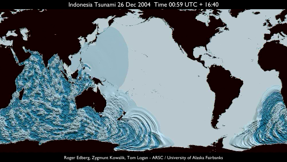
Figure-movie 4.2 Global Ocean, Indonesia tsunami Dec.
26, 2004 animation.
<Click HERE to watch movie
(global-flat-titled-retime02b_small.mp4)>
Kuril Pacific Tsunami Propagation, 2006
The movie below (Figure-movie 4.3), depicts propagation
of tsunami in the North Pacific in November 15, 2006. The source function, i.e.,
the bottom uplift/downdrop has been described in Fig. 4.22 of the text. The
movie shows wave propagation for 14-hour time span. Initial bottom uplift
generates two wave-systems, one traveling to the North-West into the
Okhotsk Sea and the second wave propagates to the South-East towards Hawaii.
The wave moving to the North Pacific is transformed by the large bathymetric
features like Emperor Mountain Chain, Hess Rise, Koko Guyot, Hawaii Island and
Mendocino Escarpment. The focusing by Mendocino Escarpment and Koko Guyot brings
large waves to Crescent City, often a few hours after the first wave
arrival. Time comparison between the measured sea level by two DART Buoys
and computed by the model demonstrates that only the first few waves are well
reproduced. Later arriving waves are badly reproduced due mainly to the
coarse resolution bathymetry used in computations.
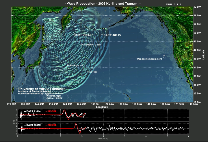
Figure-movie 4.3 Kurile tsunami Nov. 15, 2006
animation.
<Click HERE to watch movie (Northpac_kurile_small.mp4)>
Kuril Energy Flux
To
further identify Koko Guyot as an important bathymetric feature, the non-linear
shallow water wave equations were solved numerically on a 1 arc-minute grid and
used to compute energy flux vectors in time. These are defined by Eqn. 1.52 in
the text. A main energy lobe (first wave front) is observed once the tsunami
wave arrives at Koko Guyot. A later circular expanding wave front, clearly
centered on Koko Guyot, is seen to be scattered by the seamount. In this way,
two closely spaced wave fronts are observed over the Northern Pacific. These
are further enhanced by the Mendocino Escarpment. The two maxima can be easily
tracked up to their arrival at Crescent City.
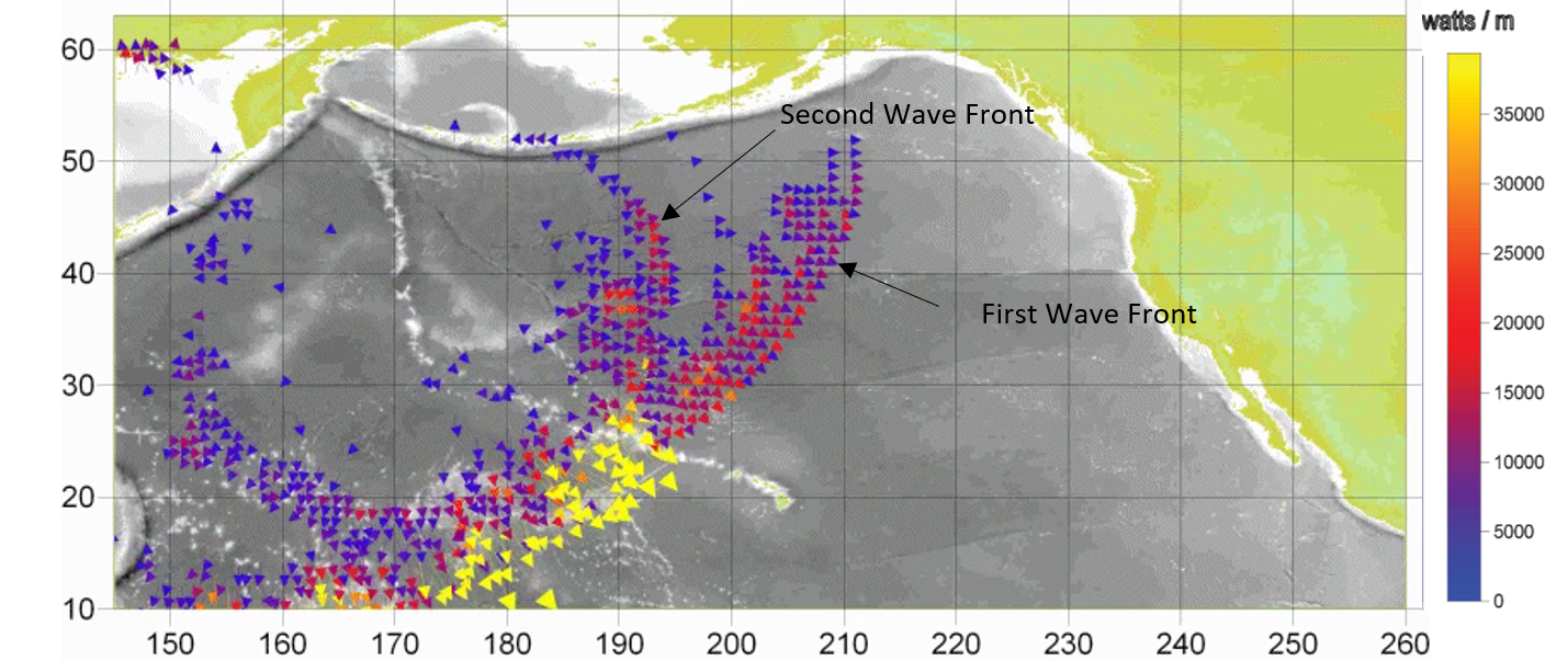
Figure-movie 4.4 Kurile tsunami energy flux animation.
<Click HERE to watch movie (kurile_energyflux.mp4)>
Guyot_inset:
Scattering dynamics are
explored in more detail in a simplified 2D model geometry using Cartesian
coordinates and the linearized shallow water wave equations. Coriolis terms
were not included. The model domain is a 400 km X 400 km square at 1 km
spatial resolution. The “ocean” bathymetry is flat at 5000 m depth. The guyot
(a crude approximation of Koko Guyot) is a right cylindrical frustum with base
radius equal to 60 km, located at the center of the model domain. The top, at 500
m depth, has a radius of 40 km. A 1m amplitude plane wave with 75 km
wavelength and moving in the +x direction is incident on the guyot (Figure-movie 4.5)
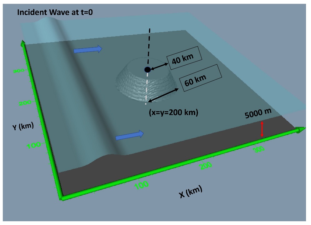
Figure-movie 4.5 – Guyot
model geometry at t = 0.
<Click HERE to watch movie (Guyot_inset.mp4)>
Snapshots of the sea
surface at defining moments are shown below in Figure-movie 4.6.
The circular
expanding wave front in Figure-movie 4.6, is identified as the scattered wave.
The angular dependence of the energy flux (defined by Eqn. 4.10 and 4.11 in the
text) is defined as the maximum energy flux passing through a circular
mathematical surface of radius 250 km, centered on the point (x=340 km, y = 300
km). This point is located on the downwind edge of the guyot. The domain size
was increased to 600 km X 600 km in order to better separate the incident and
scattered wave fronts.
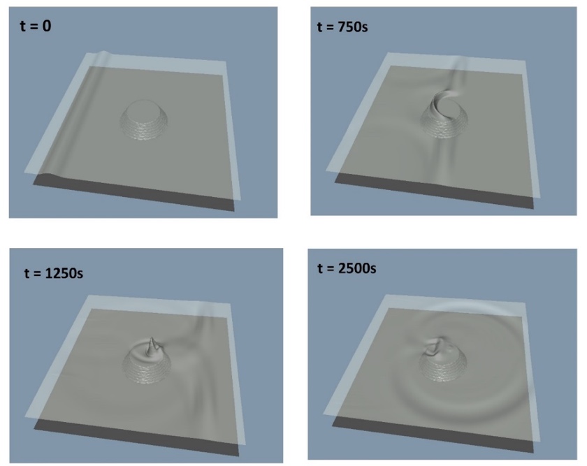
Figure-movie 4.6 – top_left:
prior to wave / guyot interaction, top_right: refraction around top of guyot,
bottom_left: Max amplitude spike at downwind side of the seamount,
bottom_right: the slower wave atop the seamount, moving in the -x direction,
wraps around the guyot, producing a nearly circular expanding wavefront.
The plot in Figure-movie
4.7 below shows the normalized scattering amplitude as a function of scattering
angle. In this example the amplitude is the maximum energy flux passing through
a circular mathematical surface of radius 250 km, centered on the point (x=340
km, y = 300 km). The scattered energy flux amplitudes are normalized to the
incident wave value. Scattering towards Crescent City would be roughly at q = 100 -110 degrees
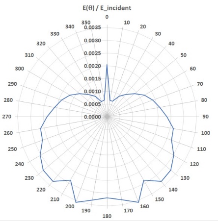
Figure-movie 4.7 – Maximum
energy flux as a function of scattering angle. Theta = 0 corresponds to
propagation in the -x direction. The flux is normalized to the incident wave
energy flux
Chapter V – SECTION 5.2
shelf break / trapping
NARRATIVE -
CONNECTION TO THE TEXT
Ch.V, Sec.2 considers two
cases of tsunami running onto the shelf – the linear sloping bottom and a more
realistic shelf profile from the Gulf of Alaska. These interactions resulted
in reflected waves and trapped wave oscillations over the shelf. And as we see
in Ch.IV descriptions of the Indian Ocean and the Kurile Islands tsunamis, the
main reason for modifications of transoceanic wave propagation is the
interaction of waves with bathymetric features such as shelves, oceanic ridges,
and seamounts. This simple animation shows how the shelf break generates these
behaviors.
Model Description
·
The
animation depicts the effect of a simple (sharp) shelf break on an incoming
single wave, revealing trapping, reflection, and transmission of wave shape
across a simple bathymetric discontinuity.
·
This
is a 1D, transient shallow water wave model u (x, t) and ζ(x, t)
– with no non-linear terms
·
Spatial
step size ∆x is 1 km, time step is 1 s.
·
Position
along the x axis is denoted by x = ∆x * i where i = 1, 2, 3,
4, …….., 1000
·
The
shelf break transition occurs within a single spatial step at i = 600. Note
that the results are nearly identical if the transition occurs linearly over 5
steps ( 598 < i < 604).
·
300
animation frames were generated at 100 s intervals - giving 8.3 hours of wave
evolution
·
The
initial wave form is the positive half of a sinusoid with λ= 200 km and ζ
(x, 0) = SIN(2πx/ λ) for 0 < x < 100 km, and ζ (x,
0) = 0 elsewhere
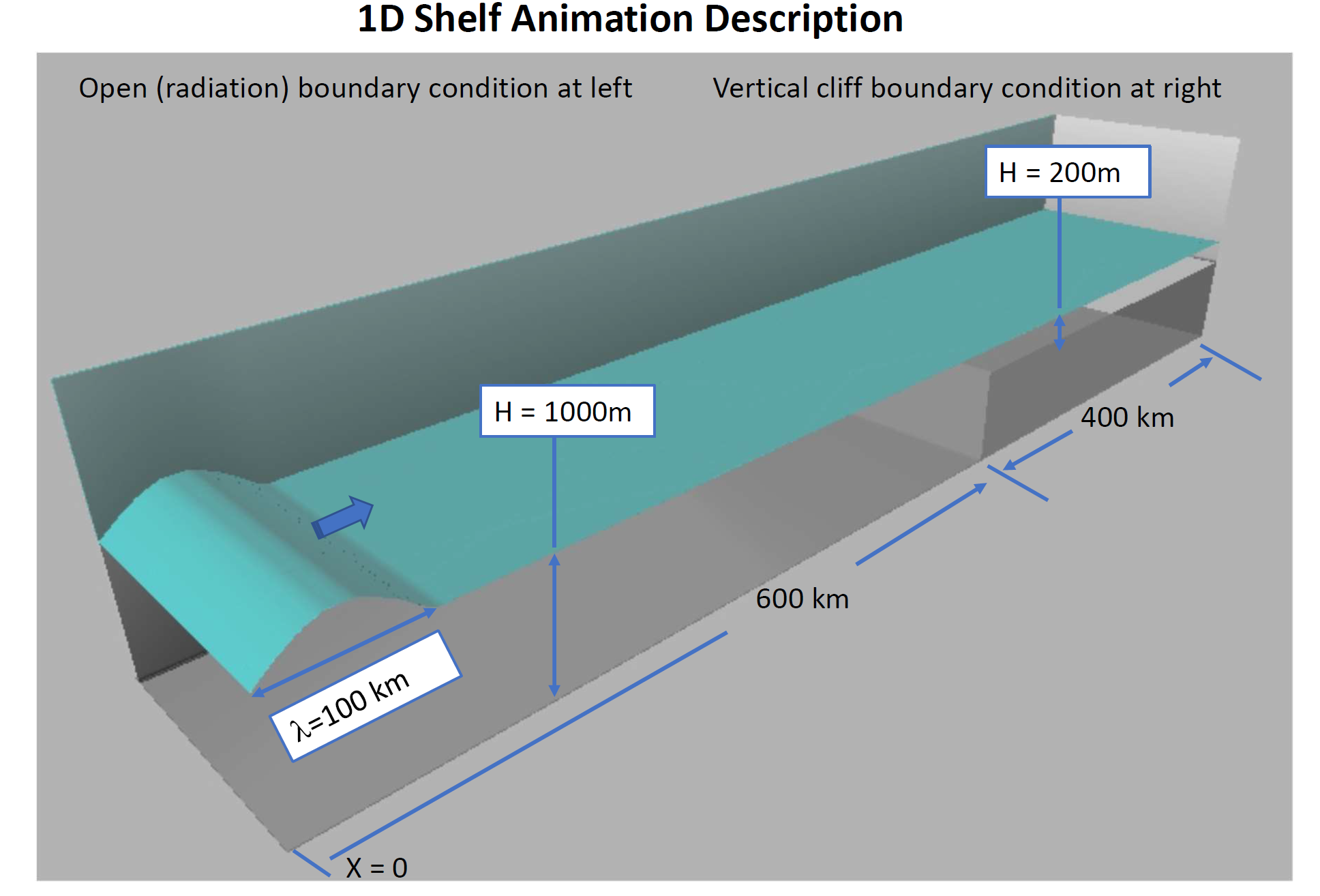
Figure-movie 5.2.1 –
Wave trapping and reflection by a continental steep shelf break.
<Click HERE to watch movie (ShelfBreak.mp4)>
Model summary
Sea level time
series for two “numerical gages” (blue is taken at i = 400 in deep water
and red
at i
= 650 in shallow shelf water). Note that the transmitted and reflected wave
amplitudes track well with predictions in Chapter 2, sec 1 Fig 2.2 and
eqn 2.7
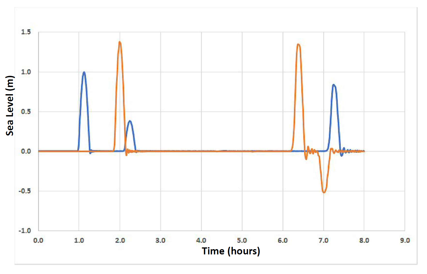
Figure-movie 5.2.2 –Transmitted
and reflected wave comparison. Deep water (red)
and shallow water (blue).
Chapter V - SecTION 5.2
IMPLICATIONS OF RUNUP
NARRATIVE -
CONNECTION TO THE TEXT
The
tsunami traveling towards the shoreline interacts with the bathymetry. The
shallow water slows the tsunami signal down, magnifying its amplitude and
velocity. We consider the linear profile given in Figure 5.1 of the textbook
(Figure-movie 5.2.3).
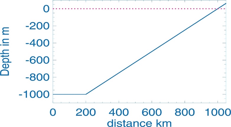
Figure-movie 5.2.3. Linear bottom profile.
The
tsunami is generated by the uplift of a 100 km long segment of ocean bottom
between 50 and 150 km from the open boundary at a depth of 1000 m. The initial
wave height is 200 cm, and as the wave propagates to the open boundary and to
the sloping bottom, it splits into two waves of 100 cm. The initial boxcar
signal profile traveling up slope undergoes two changes; its wavelength
steadily shortens, and its amplitude grows. Arriving at the shoreline, it
generates a runup. The reflected wave from the shoreline lost its boxcar
profile and resembled an oscillatory wave, see Figure-movie 5.2.4.
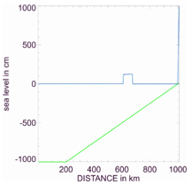
Figure-movie 5.2.4. Transformation of a square tsunami wave
on an upslope channel
<Click HERE
to watch movie (Tsunami.mp4)>
The
wave traveling towards the open boundary undergoes similar transformations as
the boxcar signal. However, in reverse order, i.e., the large amplitude
diminishes, and the wavelength continuously increases while the wave propagates
toward the left open boundary.
This
experiment shows the importance of bathymetry in generating reflected (secondary)
tsunami signals. The periods of the secondary waves are defined by reflection
and by the generation of new modes of oscillations through an interaction of
the tsunami waves with the shelf/shelf break geometry. The previous movie (Figure-movie
5.2.4) shows
the tsunami traveling 800 km upslope and downslope in the channel. The next
movie (Figure-movie 5.2.5) describes domain located between 980 km and 1010 km,
where channels changes from water to 50 m on land (dry domain).
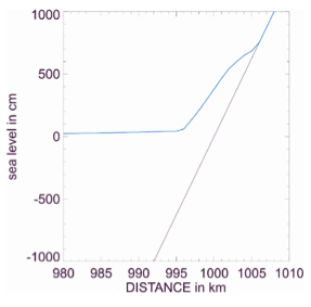
Figure-movie 5.2.5. Transformation of a square tsunami wave
on an upslope channel
<Click HERE to watch movie (Tsunami
runup and rundown.mp4)>
The
detailed process of wave amplification when it travels up and down the beach
can be observed. The domain and the runup of 8.5 m amplitude and rundown of
-5 m are shown in Figure-movie 5.2.6
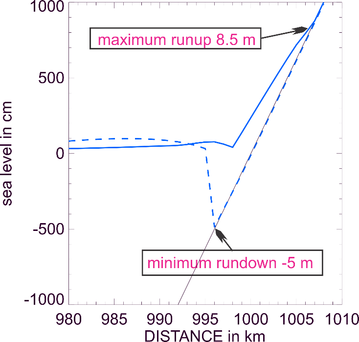
Figure-movie 5.2.6 Tsunami traveling up the beach (8.5 m)
and down the beach (-5 m). This is the upper part of the channel depicted in
Figure-movie 5.2.3
Model Description
The one-dimensional models from Chapter 1 serve as a
base for the present experiments on tsunami propagation and runup. The equation
of motion includes all terms, and only Coriolis force is neglected. The
Fortran program developed for the runup study titled: runup_beach.f90 (see the textbook,
page 93) has been modified to include tsunami generation. In the original
program, the wave enters the channel through the left open boundary. In the
modified program, the radiation condition governs this boundary. When the
bottom uplift generates a tsunami, the wave moving to the left is radiated
outside by this condition. The spatial grid of 10 m resolves the wave in the
channel of 1000 km (100000 grid points). The boxcar tsunami signal of 100 km
long is well resolved, but the boxcar is not a sinusoidal signal. It is
important to resolve the steep front and back of such a signal. Practically,
one can always expect some dispersive waves at both ends. This process is
stronger in shallow water. Figure-movie 5.2.7 describes the enhancement and the
changes at both ends of the boxcar signal in the channel. The wave arriving
at the beach reveals even stronger deformation (Figure-movie 5.2.8). The
question is why the front of the wave is much less distorted than the back. In
shallow water, along with the dispersion, the total depth (which includes both
depth and sea level) changes the wave speed at the bottom and the top of the
signal, thus resulting in additional deformation.
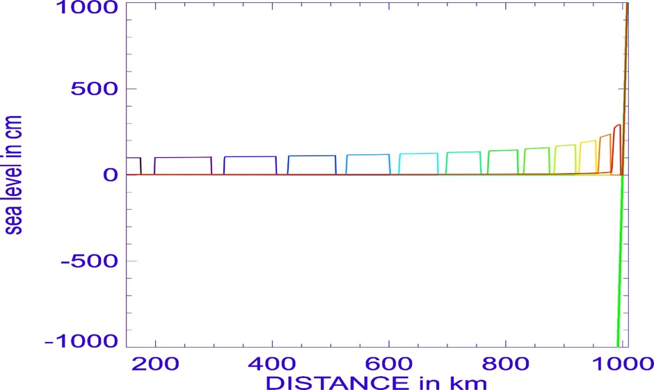
Figure-movie 5.2.7
The amplification and distortion of the boxcar signal. Different colors show
the movement of the signal toward the shore.
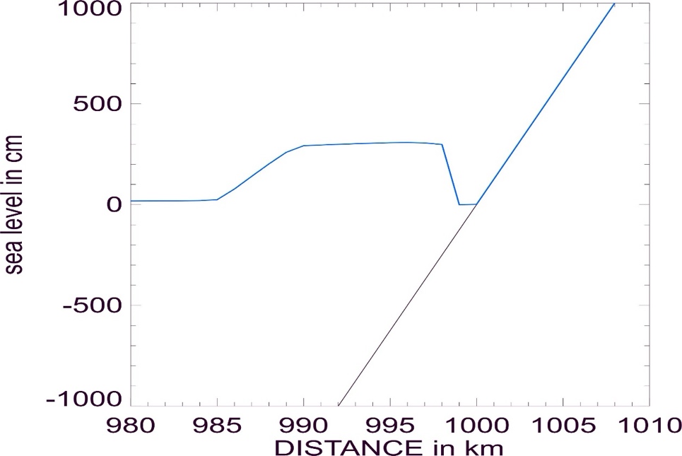
Figure-movie 5.2.8
Tsunami in close proximity to the beach. The front and the back of the boxcar
signal show different distortion.
Model summary
This experiment shows the importance of bathymetry in
generating reflected (secondary) tsunami signals. The periods of the secondary
waves are defined by reflection and by the generation of new modes of
oscillations through an interaction of the tsunami waves with the shelf/shelf
break geometry. The boxcar tsunami signal interacting with
the sloping bottom generates oscillatory signals of different shape from the
initial boxcar. The distortion at the front/back of the wave could be
attributed to a combination of shoaling (at the front of wave), reflection and
dispersion (at the tail of the wave).
Chapter V - SecTION 5.7
IMPLICATIONS OF shelf break MORPHOLOGY
NARRATIVE -
CONNECTION TO THE TEXT
Chapter 5, Sec.5.7
considers the effect of both shelf and coastal configuration centered on
Crescent City, CA. Due to their curvatures, wave trapping, focusing and its resulting
amplification are possible. This animation shows how a simple curved shelf
break can produce both amplification and modulation of maximum wave amplitudes
along a simple straight coast.
MODEL
DESCRIPTION
● This is a 2D,
transient shallow water wave model u(x, y, t), v(x, y, t), and ζ(x,
y, t) – with no non-linear terms
● The spatial step
sizes ∆x and ∆y are 1 km. The time step is 1 s.
● Position along the x
and y axes is denoted by xi = ∆x * i where i = 1, 2,
3, 4, …….., 500 and yj = ∆y * j where j = 1, 2, 3, 4,
…….., 500
● 150 animation
frames were generated at 200 s intervals - giving 8.3 hours of wave evolution.
● The initial right
moving wave is the positive half of a sinusoid, where
ζ (x, 0) = a*SIN(2πx/ λ)
for 0 < x < 160 km, and ζ (x, 0) = 0 elsewhere. The
amplitude a is 0.25m, and λ= 320 km
● The shelf break
(see figure-movie 5.7.1) is parabolic in shape according to  with a central “bulge” h of
150 km. Ly is the domain width (500 km). The abrupt transition from
1000m to 62m depth is smoothed over 2∆x. Considered as a lens,
the apparent focal length (FL) is seen in the model results to be ~310 km.
This analogy can only be approximate because a true focus would produce an
extremely tall and steep mound of water- which would expand radially prior to
reaching that point.
with a central “bulge” h of
150 km. Ly is the domain width (500 km). The abrupt transition from
1000m to 62m depth is smoothed over 2∆x. Considered as a lens,
the apparent focal length (FL) is seen in the model results to be ~310 km.
This analogy can only be approximate because a true focus would produce an
extremely tall and steep mound of water- which would expand radially prior to
reaching that point.
● An interesting
aside is that treating the shelf break as a lens and using Snell’s Law with  playing the role of index of refraction
gives results similar to the model. FL in this case varies somewhat along the
length of the shelf break, but within 125 km of the domain centerline, the FLs
are between 280 and 330 km, bracketing nicely the model results.
playing the role of index of refraction
gives results similar to the model. FL in this case varies somewhat along the
length of the shelf break, but within 125 km of the domain centerline, the FLs
are between 280 and 330 km, bracketing nicely the model results.
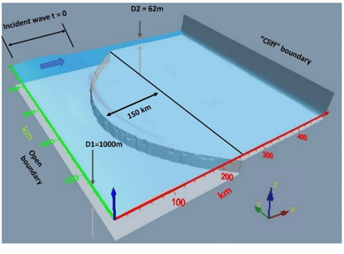
Figure-movie 5.7.1 Convex
shelf break and straight cliff boundary
<Click HERE to watch movie
(ShelfBreakMorph.mp4)>
MODEL
SUMMARY
In this animation (Figure-Movie 5.7.1), the shelf break
has curvature while the coast is straight (x = constant= 500 km). During the
time leading up to coastal impact and 1 hour following reflection back towards
the shelf break, the maximum wave amplitude occurs along the domain centerline
at y = 250 km. The tan-colored mathematical cut-plane (x-z plane) seen
in the animation is placed at the model centerline to display the wave profile
more clearly. Model results are also depicted in Figure-movie 5.7.2, showing
the effect of wave focusing on amplitude and resulting impact at the coast.
In the absence of shelf curvature, the modeled coastal
impact would be uniform across the length of the coast. Prior to arrival
however, the wave front is curved such that the first impacts occur close to
both coastal edges which then move towards the center of the coast over a
period of 41 minutes. This can be seen in the animation as what appears to be
a pair of diaphanous waves moving along the coast and converging at the
center. Figure-movie 5.7.3 shows this wave arrival dependence on time and location.
Note the gray curve corresponds to the moment of maximum coastal amplitude.
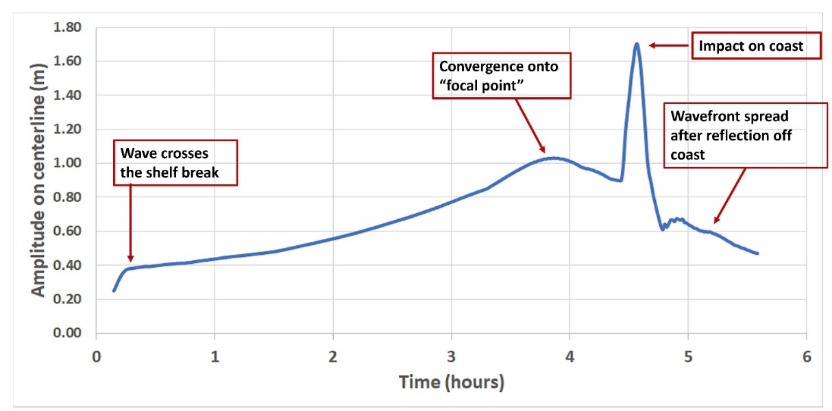
Figure-movie 5.7.2
Maximum wave amplitude at y=250 km
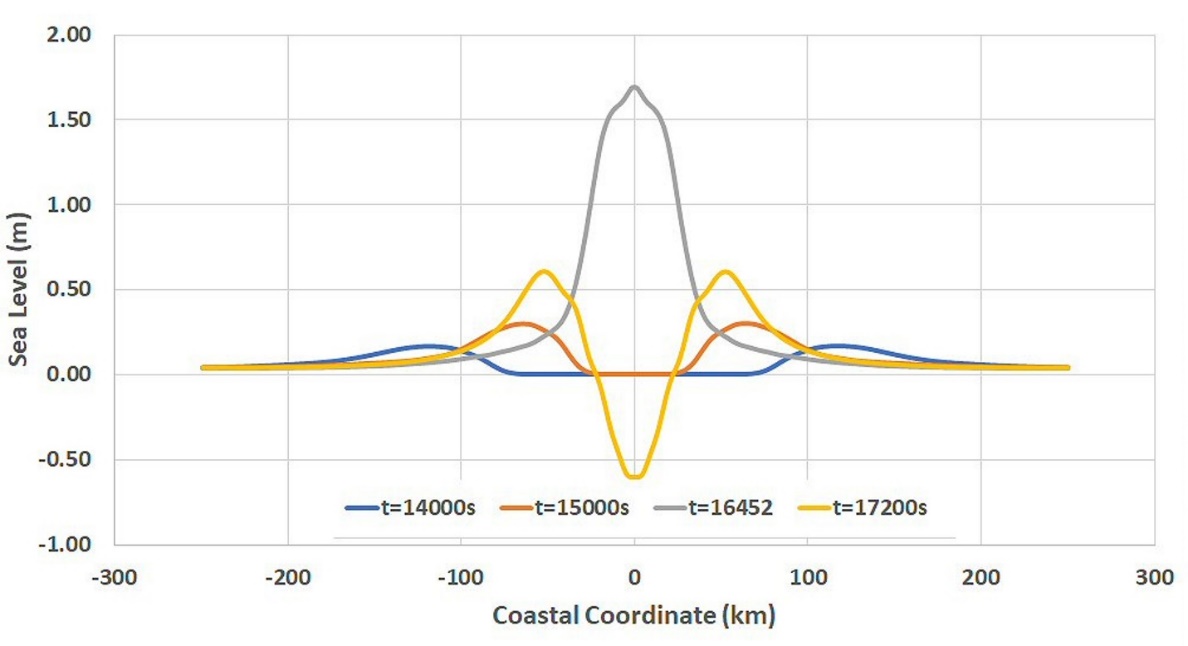
Figure-movie 5.7.3 Coastal
impact (coastal coordinate as measured from centerline)
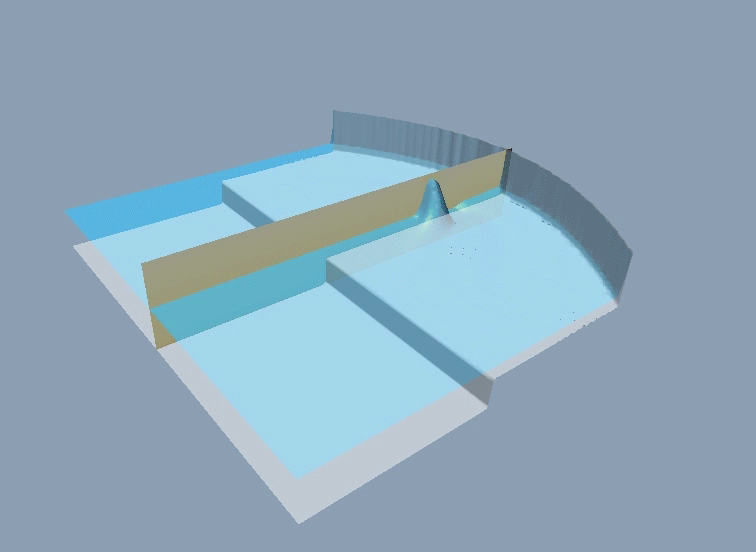
Figure-movie 5.7.4
Straight shelf break and concave cliff boundary.
<Click HERE to watch movie (Reflector.mp4)>
The animation (Figure-Movie 5.7.4) shows an interesting
reversal of the original model geometry where shelf break and coastal details
have been interchanged. The coast now has curvature while the shelf break is
straight and oriented perpendicular to the incident wave. The remaining
parameters are unchanged. Note that there is a similar focusing behavior due
not to refraction in this example, but to coastal reflection. Figure 5.14 of
the text displays bathymetry near Crescent City, California that contains
elements of both animations – curvature of both coastline and shelf break.
TSUNAMIS
AND GEOMETRIC OPTICS
NARRATIVE - CONNECTION TO THE TEXT
Section 5.7 also
introduces rays into the explanation of wave periods observed at
Crescent City, California. In this context, each length element of a wave
front is considered to have a ray associated with it - a 2D vector
perpendicular to the local wavefront and parallel to the direction of
propagation. Its magnitude can be thought of as the local phase velocity.
Rays, a concept found in geometric optics, have remarkable predictive utility
in understanding shallow water wave propagation. They are also useful in many
qualitative predictions of tsunami wave behavior. Their close connection to
tsunamis is demonstrated in this animation of wave propagation in an “ocean” of
uniform depth. The coastline, shown in figure-movie 5.7.5, is
elliptical with semi-major axis of 480 km (Xm) and semi-minor axis of
400 km (Ym). The two ellipse foci are located at y=0, x=+-265km. A ray, drawn
in red, leaving the left focus, is reflected to the right focus (anticipating θi= θr). The sum of the two path lengths is a constant for any coastal
point. This results in all rays departing the left focus at t=0
converge simultaneously on the right focus, leading to wave reinforcement.
These analytical results provide a useful model test.
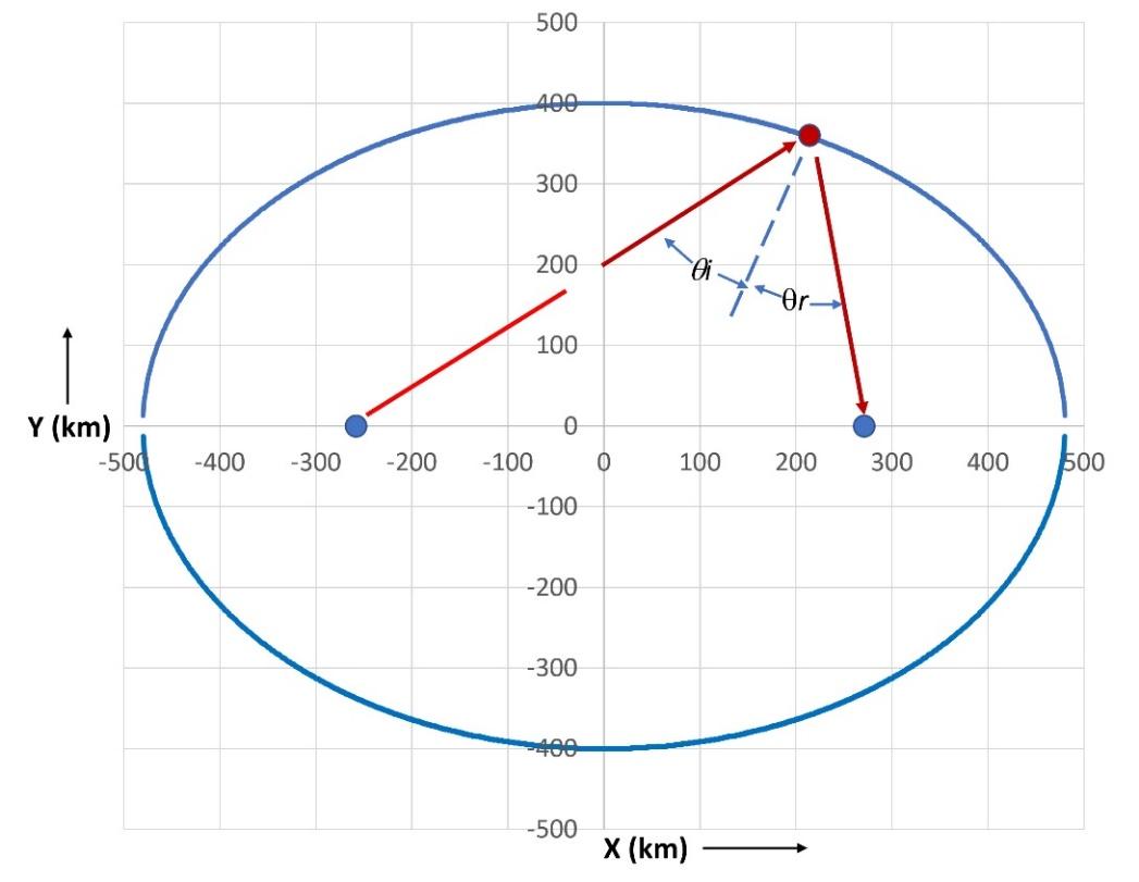
Figure-movie 5.7.5-
model geometry and representative ray path
ELLIPTICAL
OCEAN MODEL DESCRIPTION
● This is a 2D,
transient, shallow water wave model, with variables u (x,y, t), v(x, y, t),
and ζ(x,y, t). Non-linear terms, friction, and Coriolis forces have not
been included. The model is developed in the Cartesian system of coordinates.
● Spatial step sizes ∆x
and ∆y are set to 1000 m, and the time step is 1/2 s.
● “Ocean” depth is
uniform at 5000m, giving a wave phase speed  of 221 m/s
● Position along the x
and y axes is denoted by x = ∆x * i where i = 1, 2, 3, 4, ……..,
1000 and y = ∆x * j where j = 1, 2, 3, 4, …….., 1000
● Initial
conditions are:  . Setting
  ,
,


where Ao = 40 m
and ro = 40 km
The coastal equation for
the model ellipse is

● 85 animation frames
were generated at 100 s intervals - giving 2.4 hours of wave evolution. This
allows the initial sea level disturbance to transit from left to right focus
and back again to the left focus starting point.
MODEL
SUMMARY
Snapshots of the wave
propagation from the source at the left focus to first arrival at the right
focus in shown below in Figure-movie 5.7.6
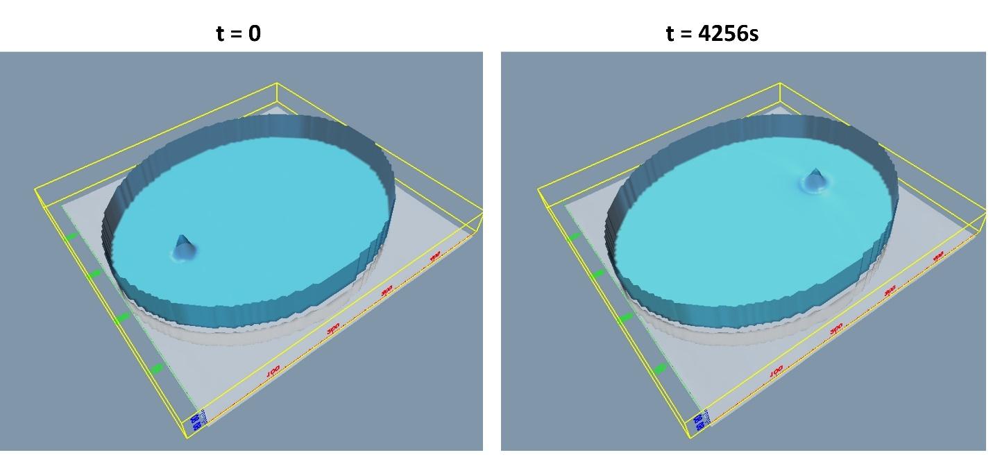
Figure-movie 5.7.6:
Maximum Amplitudes at two foci – source located at left focus
<CLICK HERE TO WATCH MOVIE (Ellipse.mp4)>
The analytically derived prediction has the initial
source disturbance converging onto the right focus, located at y = 0, x=265
km. The model result is identical to within the 1 km grid resolution. The
expected wave travel time between foci is  . The model result for travel time
to maximum amplitude at the right focus is 4256s – an under-prediction of
1.8%. Model plots of sea level taken along the x-axis,
. The model result for travel time
to maximum amplitude at the right focus is 4256s – an under-prediction of
1.8%. Model plots of sea level taken along the x-axis,  , in Figure-movie 5.7.7 clearly show
the presence of dispersion. A more pronounced dispersive tail develops during
the second transit from right focus back to the left focus.
, in Figure-movie 5.7.7 clearly show
the presence of dispersion. A more pronounced dispersive tail develops during
the second transit from right focus back to the left focus.
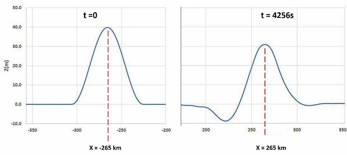
Figure-movie
5.7.7 Maximum Amplitudes at two foci
AN
EXPERIMENTAL RESULT
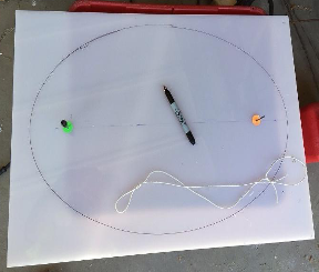
Figure movie 5.7.8
-Experimental Elliptical Tank
CLICK HERE TO WATCH MOVIE (EllipseMovie_2.mp4)>
A simple physical model with elliptical geometry was
constructed from plastic parts in a garage (figure 5). The semi-major axis is
28 cm and semi-minor axis is 19cm. The tank was flooded to 3 cm depth with tap
water. Colored sticky dots locate the two foci. A movie of wave motion from
left focus to right can be seen by clicking on the link below. Motion can be
seen continuing through several cycles.
NARRATIVE -
CONNECTION TO THE TEXT
Analysis of the
data recorded during the Indian Ocean Tsunami of December 2004, and Japan
Tsunami, 2011 demonstrated that the tsunami waves were noticeably dispersive. As
the initial wave propagates, separation of the wave into spectral components
with different frequencies and amplitudes occurs. Thus, the leading wave is
followed by a train of waves formed in its wake. This train of waves interacts
in coastal regions with the leading wave runup, drawdown, and reflection from
shelf or from land, introducing strong modification to leading wave effects.
Model DescriptionS
To show the dispersive
properties of tsunami and the limitations of the nonlinear shallow
water (NLSW)
approach, three different models are compared: NLSW, nonlinear Boussinesq
(NLB) and full Navier-Stokes equation aided by the volume of fluid method (FNS-VOF).
Small domain encompassing the south part of the Bay of Bengal is used for the
numerical simulations. Comparisons are made between NLB and NLSW models to
uncover dispersive effects.
Figure-movie 6.1
shows the wave pattern at time 1 h 40 min using nonlinear shallow water (NLSW)
and nonlinear Bousinesq (NLB) approaches. Due to dispersion effects, the NLB
model features a pronounced series of waves trailing behind the leading wave.
The wave pattern is significantly different from that of the NLSW model. From
the NLB model results, it is seen that the length of the wave train is longer
in the western region than in the eastern region (close to Thailand and
Indonesia).
As Eqs. (6.1),
(6.2) and (6.3) suggest (Chapter 6, Sec. 6.2.2), the magnitude of the
dispersive term is proportional to the square of the water depth, and therefore
the dispersion effect in the western region (H = 4 to 5 km) is much stronger
than in the eastern region (which is only of several hundred meters deep).
Dispersive effects are also enhanced in the western region by the greater distance
of propagation. Table below (textbook 6.2) gives model setup information and
computer performance on a PC desktop single CPU computer (2006).
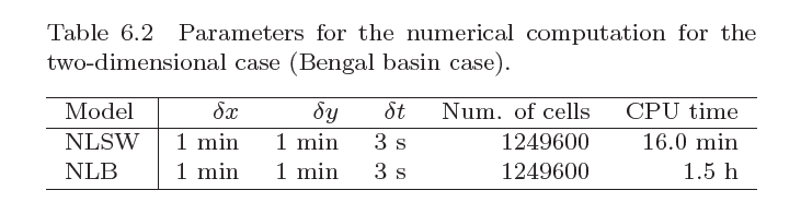
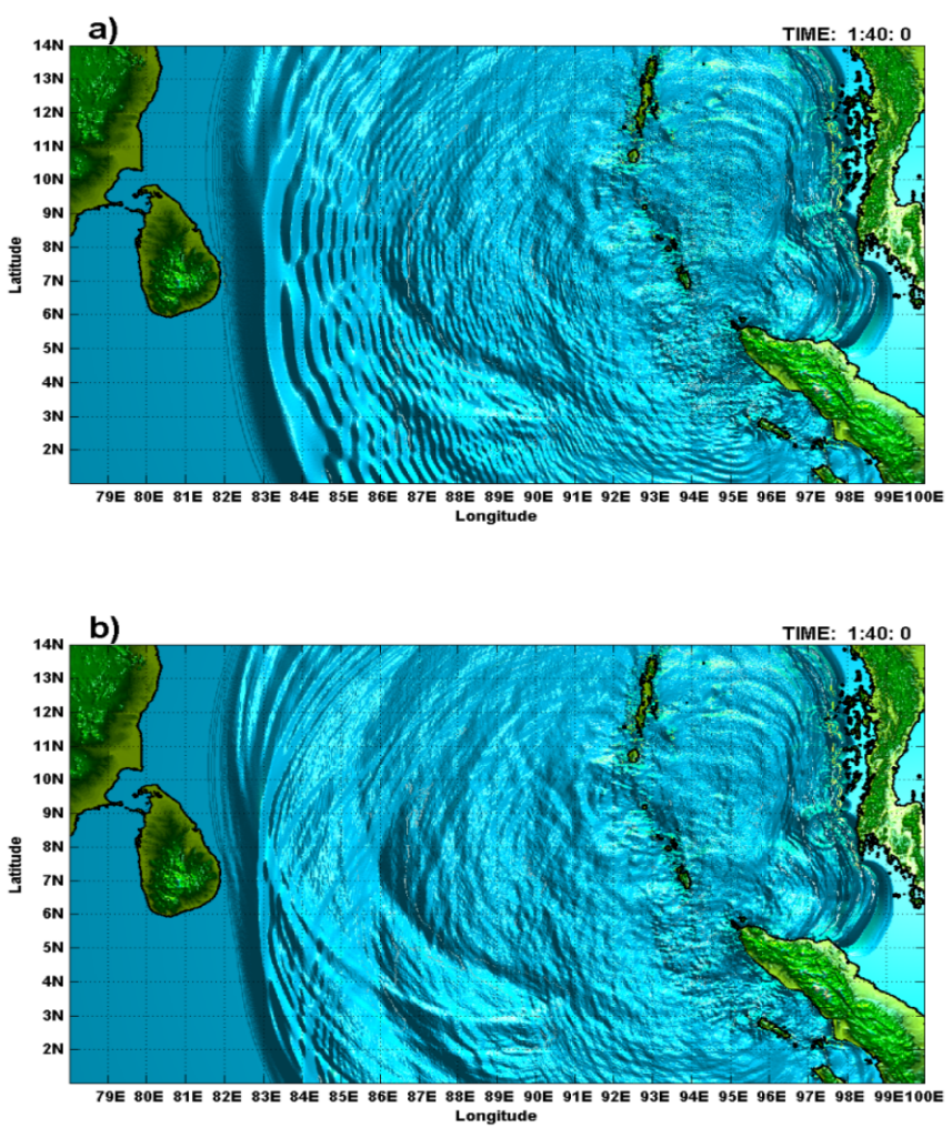
Figure-movie 6.1 Comparison
of water surface computed at 1 h 40 min from the onset of the earthquake: a) 2D
NLB model results, and b) 2D NLSW model results
<Click HERE to watch movie (NLSW_NLB_small_new.mp4)>
A simplified
additional study is incorporated in which one-dimensional channels are used
again to reveal the dynamics of dispersive wave runup. Model setup for this
study is given in the following table
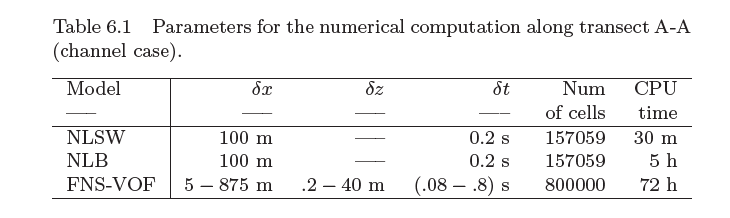
Figure-movie 6.2
shows the free surface snapshot at time 1 hour 20 min (4800 sec) from the onset
of the earthquake of the Indian Ocean Tsunami (IOT) by three numerical models, 2D
Full Navier-Stokes (FNS), 1D NLB and 1D NLSW. The IOT propagation is based on the
initial free surface deformation given by Fig. 3.9 of the textbook. General
features of the wave evolution agreed very well in all approaches. However,
some differences in reproducing the dispersion phenomena become noticeable as
time advances (see movie). For instance, at time 40 min (2400 sec), wave
dispersion is evident in the NLB and FNS-VOF results. A train of waves,
imparted by the multiple frequency components of the leading wave, is formed
just behind the leading wave. However, major wave features are well reproduced
by the NLSW with the exception of the trailing wave train. The leading wave is
taller and shifted forward in space relative to the dispersive approaches. The
nondispersive NLSW approach overpredicts wave height. A slight advance in time of
the NLSW leading wave crest is observed as well. However, the tip of the wave
front of the NLSW leading wave matches very well with its dispersive
counterparts. This reaffirms the use of NLSW as an accurate candidate for
determining the tsunami arrival time.
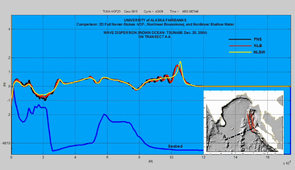
Figure-movie 6.2
Comparison of water surface computed by three models (2D Full Navier-Stokes
(FNS), 1D NLB and 1D NLSW) at 1 hour 20 min (4800 sec) from the onset of the
earthquake. Notice that the time plot is running in the opposite direction.
<Click HERE to watch movie (CASE_0015New1.mp4)>
Model summary
Comparison of the
three different methods shows that for practical purpose the NLSW model results
are quite reliable since this model gives consistent results with its
counterparts. The NLSW approach is very attractive nowadays for tsunami
calculation because this method has very low computational cost. In addition,
maximum wave height and runup are often overpredicted, increasing the safety factor.
The NLSW results are useful for preliminary hazard assessment, where a simple
and quick estimation of maximum wave height, maximum run-up, and locations of
maxima are required. Accuracy of location of the wave front tip for the IOT is
excellent, reaffirms its use as a method for determining the tsunami arrival
time. Qualitatively and quantitatively, the wave fronts reproduced by the NLB
and FNS-VOF solutions share many common features. For longer integration times,
the similarity holds only for the main maximum, because the phase difference
between secondary maxima increases with travel time.
Chapter VII
Simplified VOF (Volume of Fluid) Free SurFace
RECONSTRUCTION For the DAM-BREAK PROBLEM
NARRATIVE -
CONNECTION TO THE TEXT
Modeling complex surface or interface evolution
requires techniques that deal with multiple phases or separation of fluid. Examples
which facilitate the understanding of these techniques include simulation of breaking
waves or dam breaking. For these simulations the full Navier-Stokes and
continuity equations are to be solved which also include the pressure field
variable, in addition to the velocity field. The free surface or interface
tracking is described by the discrete VOF function, and the fluid is advected as
a Lagrangian invariant. In our notation this is the function F, see Chapter VI
p. 268 and Chapter VII p. 322
Model Description
·
This
is a 2D time dependent Navier-Stokes model u (x,z,t), w (x,z,t)
and F(x,z,t). Spatial step size ∆x is 1 cm, ∆z is 0.5 cm and
time step is 0.01 s.
·
The
inclusion of the vertical direction in the physics is an improvement for the
solution of the dambreak problem as is the inclusion of the pressure
·
Domain
size is 40 cm by 20 cm
·
The
initial dambreak free surface is defined as step function at t=0
·
The
animation depicts the determination of the F function in time
Model SUMMARY
In this particular 2D dambreak
case, the standard VOF method of Hirt and Nichols [1981] for tracking the
evolution of fluid interface has been simplified to clarify its concept. Here,
only the concentration of the fluid (F) is determined by using the transport
or concentration equation at each of the computational grid or cell. A value of
F=1.0 (dark blue) indicates a full filled cell and value of F=0 (white)
indicates an empty cell and a value 0 < F < 1 indicates a surface cell (blue
saturation). The surface interface (black line) is calculated by merely using a
contour line at the value of 0.5. This is the simplest approach for surface
reconstruction using the VOF method.
Figure-movie 7.1 Simplified
surface reconstruction for the 2D dambreak problem using contour line of
F=0.5.
<Click HERE to watch movie (CASE_0095_new.mp4)>
Model Description
·
This
is a 2D wave propagating into the shore over a mild slope generating a plunging
breaking wave. The time dependent Navier-Stokes model includes u (x,z,t),
w (x,z,t) and F(x,z,t) and p(x,z,t). Pressure is obtained by
solving the Poisson equation using a iterative solver (incomplete Cholesky
conjugate gradient method) of the resulting linear system of equations. Spatial
step size ∆x is 1 cm, ∆z is 0.5 cm and time step is 0.01 s.
·
Domain
length is 36 m by 2 m high. The wave is generated by a piston like wavemaker
to generate a soliton of 0.45 m amplitude. The water depth along the flat
bottom is 1 m with a mild slope of 1:15 ramping up at the location x= 20 m. Here,
the inclusion of the vertical direction in physics is also important for the
solution of the plunging breaking wave.
·
The
animation depicts the wave propagation and the plunging breaking wave. Again, the
free surface is defined by the F function
Model SUMMARY
In this particular  test,
the VOF surface tracking technique proves that the solution of complex surface
dynamics is possible. However, the solution requires additional computational
resources for the solution of the pressure field.
test,
the VOF surface tracking technique proves that the solution of complex surface
dynamics is possible. However, the solution requires additional computational
resources for the solution of the pressure field.
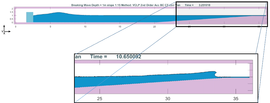
<Click HERE to watch movie (Fullscale2cm.mp4)>
<Click HERE to watch movie
(Zoom1cm.mp4)>
EDUCATIONAL
PROGRAMS
BOOK: NUMERICAL
MODELING OF TSUNAMI WAVES
<UNDER CONSTRUCTION1>

<UNDER CONSTRUCTION2>